 Test engineering
AI vision inspection in final inspection: when it pays off and how to introduce it
AI vision inspection pays off when defects are hard to describe as a fixed rule, for example scratches on textured surfaces. Success depends less on the AI models than on resolution, lighting, sample parts and clearly defined boundary samples. You show whether it is suitable with test parts that were not in the training and with separate limits for escapes and false rejects.

When does AI vision inspection pay off instead of fixed rules?
AI vision inspection pays off when a defect takes many forms and cannot be described as a fixed rule, for example scratches, inclusions or discolouration on textured surfaces. For dimensions, position, completeness with clear contrast and codes, classic image processing with fixed rules is usually enough. In many systems both methods work side by side.
Classic industrial image processing (machine vision) works with parameters: find an edge, measure a distance, count an area. This is traceable and fast. Deep learning methods learn the feature from example images. They differ in what they learn from:
| Method | Learns from | Good for | Limit |
|---|---|---|---|
| Fixed rules | parameters | dimensions, position, completeness with clear contrast, codes | many defect forms, varying surfaces |
| Classification | good and bad images for each defect type | known defect types with many examples | needs bad parts for each class |
| Anomaly detection | good images only | rare or unknown defects | reports a deviation, does not name a defect class |
Anomaly detection reports what is different, not what is defective. A new material batch or a different mould cavity can therefore produce false rejects if the good images do not cover this variation. In practice we combine both: rules for dimensions, position and code, AI for surfaces and features that are hard to describe.
What camera resolution does a vision inspection need?
The required resolution follows from the field of view and the smallest defect. As a rule of thumb from camera manufacturers, the smallest defect should cover at least three pixels, or five under difficult conditions such as low contrast. This is not a standard; two pixels are considered the theoretical lower limit.
Npx = Bdmin · k
- Npx
- required number of pixels per axis
- B
- field of view in this axis in mm
- dmin
- smallest defect to be found in mm
- k
- pixels per defect (dimensionless), usually 3, 5 with low contrast
Example: A housing with a 120 mm field of view is to be inspected for scratches from 0.15 mm. With 3 pixels per defect, this gives an image width of 2,400 pixels, so one pixel per 0.05 mm on the part. A 5-megapixel sensor with a width of 2,448 pixels is just sufficient.
What the calculation means: the pixel size on the object, here 0.05 mm, is the key figure for everything else. It determines the lens and the permissible motion blur. If one sensor is not enough, a smaller field of view with several images or a line scan camera for moving parts will help.
Typical sources of error with resolution
- Only pixels counted: the lens must also resolve the pixel size. A blurred lens turns 3 pixels into a grey spot without contrast.
- Colour camera for fine defects: the colour filter mosaic reduces the effective resolution. For surface defects, many users choose monochrome cameras.
- Codes forgotten: for 2D codes, at least 5 pixels per smallest module is the guideline. This can drive the resolution up more than the defect does.
- Contrast overestimated: a defect with 3 pixels but hardly any difference in brightness from the good area remains invisible. Then different lighting helps first, not more resolution.
Which lens and which lighting does the inspection need?
The lens follows from the magnification and the working distance: the magnification is the sensor size divided by the field of view, and the focal length follows from this and the distance to the part. We choose the lighting according to the surface and the defect type. A defect that has no contrast in the image remains invisible even to the best model.
β = sB f ≈ a · β1 + β
- β
- magnification (dimensionless)
- s
- sensor width in mm (number of pixels times pixel size)
- B
- field of view in mm
- f
- focal length of the lens in mm
- a
- object distance in mm, approximately the working distance
Example: 2,448 pixels at 3.45 µm give a sensor width of 8.45 mm. With a 120 mm field of view, β = 0.070. With a 400 mm working distance, f ≈ 26 mm. We would choose a 25 mm lens and reduce the distance to around 380 mm.
The formula is the thin lens approximation. It is sufficient for the preliminary design; the lens manufacturer's data give the exact position. Fixed focal lengths come in steps such as 8, 12, 16, 25, 35 and 50 mm, which is why the distance is usually adjusted.
Lighting by defect type
| Lighting | Shows | Suitable for |
|---|---|---|
| Diffuse front light, dome | even surface without reflections | shiny, curved parts, prints |
| Dark field | scratches and edges bright on a dark background | scratches, engravings, burrs |
| Backlight | sharp contour as a silhouette | holes, outlines, dimensions |
| Deflectometry | distortion of a reflected stripe pattern | dents and waviness on reflective surfaces |
For dimensions with tight tolerances we use telecentric lenses. They keep the magnification constant despite differences in height, but the front lens must be at least as large as the part.
How short must the exposure be for moving parts?
The exposure time must be short enough that the part moves by no more than one or two pixels during the image capture. It follows from the pixel size on the object, the permissible blur and the conveyor speed. For measuring tasks, one pixel is the better guide; some manufacturers give half a pixel.
texp ≤ pO · uv
- texp
- maximum exposure time in s
- pO
- pixel size on the object in mm
- u
- permissible motion blur in pixels
- v
- speed of the part in mm/s
Example: At 0.05 mm per pixel, 1 pixel of blur and a conveyor speed of 0.3 m/s, the exposure may be at most 167 µs.
Such short times need a lot of light. Depending on the design, strobe lighting works with a few tens to a few hundred microseconds and at the same time suppresses ambient light. If the parts are stationary during image capture, this limit does not apply, but stopping costs cycle time.
How do you calculate the cycle time budget?
The cycle time is the time available for each part. The AI evaluation often needs only milliseconds; the cycle is usually determined by feeding, positioning and the number of views.
tcycle = 3,600 sQh ≥ tfeed + nV · tV + teval + tsort
- tcycle
- available time per part in s
- Qh
- required throughput in parts per hour
- tfeed
- feeding and positioning in s
- nV
- number of views or images
- tV
- time per image including movement and image transfer in s
- teval, tsort
- evaluation and rejection in s
Example: 1,800 parts per hour leave 2.0 s per part. Feeding 0.8 s, three views of 0.2 s each, evaluation 0.1 s and rejection 0.3 s give 1.8 s. That leaves a reserve of 0.2 s. A fourth view would only be possible with a second camera in the same cycle.
Plan in a reserve. In operation, rechecks, communication with the PLC and fluctuations in feeding are added.
How does a feasibility study with sample parts work?
In the feasibility study, your sample parts show whether a feature is clearly visible in the image and can be separated from the permitted variation. This needs good parts with normal variation, bad parts for each defect type and boundary samples. Only then do we define the camera, lighting and evaluation.
- Describe the inspection task: part, inspection features, smallest defect, cycle, feeding and installation space.
- Put together sample parts: labelled as good part, defect type and boundary sample, with your assessment of each part.
- Test image capture: compare lighting types and viewing angles until every feature has contrast.
- Train and test the evaluation: with parts that were not used for training.
- Discuss the result: which features can be inspected, which only to a limited extent, and what this means for the setup and acceptance.
Example of a sample parts plan
No standard specifies fixed quantities; they depend on the feature. The following breakdown is an example for a part with three defect types:
| Group | Purpose | Example |
|---|---|---|
| Good parts | show permitted variation: batches, mould cavities, colour shades | 30 parts from several batches |
| Bad parts | each defect type in a typical form | 10 parts per defect type |
| Boundary samples | just inside and just outside the tolerance | 3 to 5 pairs per defect type |
| Test parts | testing without reference to training | separate parts that are not used for training |
The bigger hurdle is usually the question of what a defect is. In a study by Sandia National Laboratories, 82 inspectors checked precision parts for eight defect types. On average they detected 85 % of the bad parts and at the same time rejected 35 % of the good parts. If inspectors do not agree, the AI learns this disagreement too.
So before training, define a defect catalogue with images for each defect type, plus boundary samples and the person who decides on disputed parts. If there are no real bad parts, specially prepared parts help, for example with deliberately applied scratches.
How do you calculate the escape rate and false reject rate?
The escape rate is the proportion of bad parts that are rated good and go to the customer. The false reject rate, also called pseudo defects or false alarms, is the proportion of good parts that are sorted out. Both are calculated separately and need separate limits.
E = nB,goodnB F = nG,badnG
- E
- escape rate (proportion, usually given in %)
- nB,good
- bad parts that were rated good
- nB
- total bad parts tested
- F
- false reject rate (proportion, usually given in %)
- nG,bad
- good parts that were rated bad
- nG
- total good parts tested
Example: Of 300 bad parts, 3 are rated good; of 5,000 good parts, 60 are rated bad. This gives an escape rate of 1.0 % and a false reject rate of 1.2 %.
Both values depend on the same threshold. Tightening it lowers the escape rate and raises the false reject rate. Which value matters more depends on the part: for safety-relevant features it is the escape rate, for expensive parts the false reject rate. A high false reject rate also means that someone rechecks every hit by hand. A third class "Recheck" for parts close to the threshold is often worthwhile.
Convert the false reject rate into parts per shift. 1.2 % of 10,000 parts is 120 parts that someone has to look at. That is often a better argument than the percentage.
How many bad parts does the acceptance of a vision inspection need?
For a solid escape rate you need more bad parts than most people expect. If none are missed in n bad parts, the upper 95 % limit for the escape rate is still about 3/n. If you want to prove an escape rate of 0.1 %, you need around 3,000 bad parts without a single miss.
E95 ≈ 3n (with 0 missed parts)
- E95
- upper limit of the escape rate with 95 % confidence
- n
- number of bad parts tested, useful from about 30
Example: 100 bad parts without escapes only prove that the escape rate is below around 3 % with 95 % confidence. With 3 missed parts out of 300, the upper limit according to the exact binomial calculation is around 2.6 %, not 1 %.
| Bad parts without escapes | Upper 95 % limit |
|---|---|
| 50 | around 6 % |
| 100 | around 3 % |
| 300 | around 1 % |
| 1,000 | around 0.3 % |
| 3,000 | around 0.1 % |
This rule of thumb (rule of three) is the approximation of the exact binomial limit. Bad parts can be tested several times in different positions, but each test must be run with the part reinserted. Evaluating the same image several times says nothing about the variation caused by position, feeding and ambient light.
Which guideline applies to acceptance?
For classifying image processing, VDI/VDE/VDMA 2632 Part 3.1 (2020-08 edition) describes the testing of classification performance, including acceptance sampling and hypothesis testing with a sampling plan. For attributive inspection processes, VDA Volume 5 and the AIAG MSA manual name the kappa statistic. It evaluates the agreement between the inspection system and the reference assessment and subtracts the agreement that would arise by chance alone.
κ = po − pe1 − pe
- κ
- Cohen's kappa (dimensionless), 1 means full agreement
- po
- observed proportion of matching assessments
- pe
- agreement expected by chance from the proportions in each class
Example: System and reference agree on 95 % of the parts, and both classify 30 % as bad. The chance agreement is 0.3 times 0.3 plus 0.7 times 0.7, so 0.58. This gives κ = 0.88. According to the AIAG manual, values from 0.75 count as good agreement.
For acceptance, the following also applies: do not use training images, evaluate boundary samples separately and measure the cycle time over a defined number of parts under series conditions.
What does AI vision inspection cost and what does the effort depend on?
The effort is determined mainly by the number of views, resolution, surface, cycle and feeding, less by the AI software. A single view of a stationary part is a different task from an inline inspection with four cameras, sorting and traceability. We give a solid cost range after the feasibility study on your sample parts.
| Cost driver | Why |
|---|---|
| Number of views | Every side that has to be inspected needs a camera or a movement of the part. |
| Smallest defect relative to field of view | High resolution or several images per part, better lenses. |
| Surface | Shiny or curved parts need a dome, deflectometry or several types of lighting. |
| Cycle and movement | Strobe lighting, faster cameras, more computing power. |
| Feeding and sorting | Conveyor belt, separation, turning the part, delta picker, sorting outlets. |
| Variants and defect types | More inspection recipes, more sample parts, more effort for training and acceptance. |
| Verification and data | Scope of acceptance, image storage per part, connection to PLC, MES or ERP. |
Separate inspection cell or inline system?
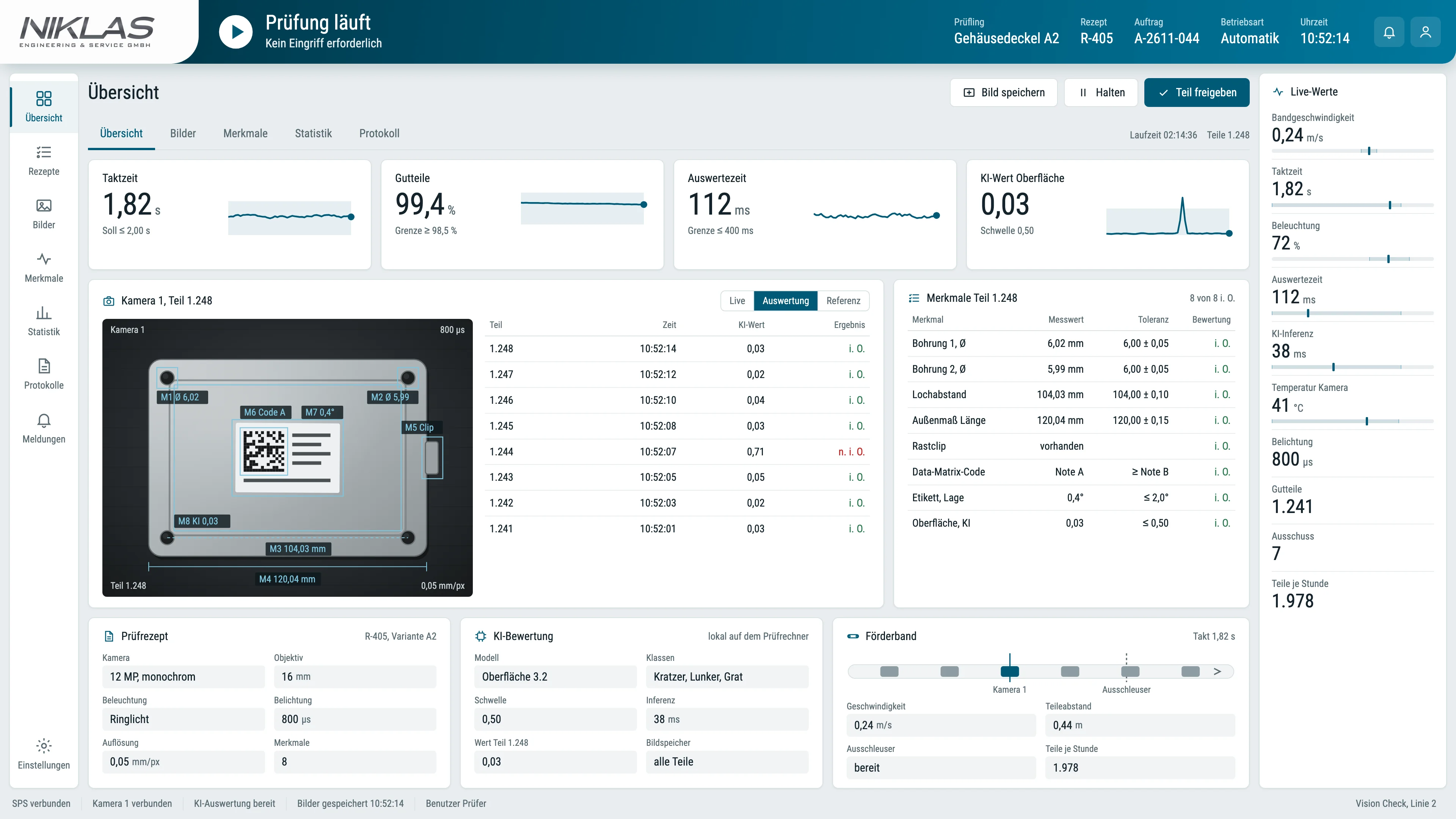
A standalone inspection cell is a good fit if parts are inspected in batches or there is no space in the line. An inline system with a conveyor belt inspects in the production flow and, with an optional delta picker, sorts directly into OK and NOK. We build both with the NIKLAS Vision Check, which is also available as a module in the modular system of our test benches.
What we need from you for a quotation
- Part with drawing or photos, material and surface
- Inspection features and defect types, with a defect catalogue if available
- Smallest defect to be found and tolerances
- Cycle or quantity per shift, number of variants
- Feeding, installation space and the interface you want to the PLC or ERP
- Sample parts, as soon as we check feasibility
Send us the details via the contact page. We will then tell you which sample parts we need for the feasibility study.
What needs attention in operation: variants, drift, data?
In operation, parts, batches and the environment change. With the Vision Check, your team creates new variants itself via the user interface. If the detection changes, check the image first: light, contamination, focus, position. Retraining only makes sense once the image is right.
A common practice is a set of reference parts that runs through the system regularly, for example at the start of each shift. If a reference bad part is not detected, that is an early sign of drift. Only release a retrained model after a new test with parts that were not in the training.
The Vision Check evaluates with locally run AI models. Inspection images and inspection data are documented for each part and can be archived for complaints. How the result gets into the test report and the ERP system is described on the NIKLAS Test Software page.
On the EU AI Act: obligations for high-risk systems are linked, among other things, to safety components of products such as machinery. In our assessment, a pure quality inspection without a safety function does not fall under this. This does not replace a legal review of the individual case.
Frequently asked questions about AI vision inspection
Answers to the questions that quality and production managers ask before an introduction.
How many sample parts do we need for a feasibility study?
That depends on the feature; no standard specifies a number. Useful are good parts with normal variation from several batches, bad parts for each defect type and boundary samples just inside and outside the tolerance. For acceptance you will later need additional parts that were not in the training.
What does AI vision inspection cost?
That depends mainly on the number of views, the resolution, the surface, the cycle and the feeding. The AI software is rarely the largest item. We give a solid cost range after the feasibility study on your sample parts.
Can we retrofit vision inspection into an existing line?
Yes, if the installation space, feeding and cycle are suitable. The Vision Check can be set up as a single cell or as an inline system with a conveyor belt and passes the inspection decision to your PLC via an interface. How the parts continue afterwards depends on your process.
Do we need bad parts if defects are rare?
Not necessarily for training: anomaly detection learns from good images. To prove that the inspection finds defects, you need bad parts. If there are no real ones, specially prepared parts with defined defects help.
What is the smallest detectable defect?
As a rule of thumb, the smallest defect should cover at least three pixels and have contrast in the image. With a 120 mm field of view and an image width of 2,400 pixels, the limit is therefore about 0.15 mm. We design the field of view, camera and lighting accordingly.
How do we prove that the vision inspection works?
With an acceptance test on parts that were not in the training, and with separate limits for escapes and false rejects. VDI/VDE/VDMA 2632 Part 3.1 describes the procedure; for attributive inspections, VDA Volume 5 and AIAG MSA name the kappa statistic. For low escape rates you need many bad parts: with no miss in 300 parts, the upper limit is still around 1 %.
Can our staff train new variants themselves?
With the Vision Check, after the initial setup your team creates new parts and inspection recipes itself via the user interface and trains new variants with good and bad samples. We define together which defect patterns are to be detected during the initial design.
Do the images leave our plant?
Not with the Vision Check: the AI models run locally on the system. Inspection images and results stay in your network and can be documented for each part.
Does our vision inspection fall under the AI Act?
High-risk obligations are linked, among other things, to safety components. In our assessment, a pure quality inspection without a safety function does not fall under this. For your individual case we recommend a legal review.
More technical articles
Test engineering Test engineering
Pump testing ISO 9906
Tolerances of grades 1B, 2B and 3B, head and efficiency with a worked example, measurement uncertainty, NPSH3 and test procedure: how a pump test to DIN EN ISO 9906 runs on the test bench. Test engineering
Test bench requirements specification
Test items, power, measurement uncertainty, cycle time, energy and acceptance with formulas and worked examples: what a requirements specification for a test bench must contain.Have your sample parts tested
Describe the part, inspection features and cycle. We will tell you which sample parts we need for a feasibility study.
Simon Niklas
Mechanical engineer, M.Sc.
+49 941 56956720[email protected]
“Good engineering proves itself in day-to-day production. That is why we combine technical planning with a close understanding of process, operation and maintenance.”
Book a consultation